Surface Interpolation for Scilabuse plot3d() and contour() with scattered data PresentationHere is a new toolbox for Scilab. This toolbox enables the use of plot3d() and contour() functions even if your data are not located on a regular grid. Indeed, a new function interpolates your data and generates automatically a regular grid. This is well suited for load-pull analysis (this example). This toolbox includes 2 functions :
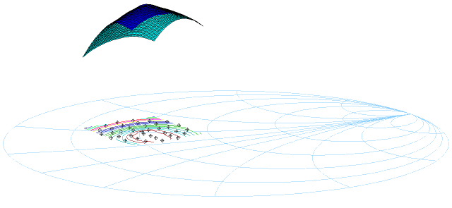
Example// This exemple displays the picture below M=fscanfMat("C:\exemple.txt"); M(:,3)=M(:,3)./1000 // Unit change from mW to W clf() ; plotsmith(12); plot2d(M(:,1),M(:,2),-8); new_data=interpolate_grid(M,10); contour(new_data(1),new_data(2),new_data(3),20); plot3d(new_data(1),new_data(2),new_data(3),alpha=28,theta=236);
Download and installation1. Download the archive file here 2. Unzip the file in your Scilab contrib directory (SCI+\contrib) 3. Launch Scilab and write the following command : exec(SCI+'/contrib/surface/builder.sce'); Now the toolbox is installed. For future scilab session, you just have to call once the surface library either by the toolbox menu or the command line : SURFACE=lib(SCI+'/contrib/surface/macros/'); |